5.14 Spatial Statistics

Spatial statistics concerns the analysis of spatially-referenced data, for instance, well locations referenced to a coordinate grid. Originally developed for soil and crop surveys and mining applications, spatial techniques are now regularly used with groundwater data. The primary goal of a spatial statistical analysis is typically map making, which involves analyzing the spatial relationships between locations and utilizing those relationships to create accurate, defensible isocontours or other maps of concentration levels and groundwater elevations. Figure 5-17 illustrates groundwater elevations that are contoured.

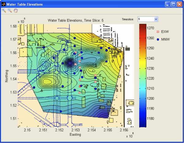
Figure 5-17. Map of contoured groundwater elevations developed in GTS using example data from the software.

Source: Example data courtesy AFCEC 2013.

For many, if not most, spatially-referenced populations — including groundwater aquifers — the possible sample values that might be collected are not evenly ‘mixed’ throughout the target area. Instead, there is likely to be a (complex) spatial stratification of the measurement levels, perhaps due to the site topography or hydrogeology, or the existence of localized contaminant sources and groundwater plumes. In addition, wells are almost never randomly located within the target area (Section 3.2.1), but are placed nonrandomly according to the dictates of the Conceptual Site Model (CSM, Section 3.2) and professional judgment.

Because of these realities, spatially-referenced observations are generally not statistically independent. Instead, there is spatial dependency or correlationAn estimate of the degree to which two sets of variables vary together, with no distinction between dependent and independent variables (USEPA 2013b). between different locations, generally meaning that chemical concentrations and/or groundwater elevations at a particular location are more similar to those at nearby locations than they are to more distant sampling points. Spatial statistical techniques are specially adapted to account for this correlation when drawing maps.

5.14.1 Spatial Interpolation and Smoothing

A common task in groundwater spatial analysis is to create a map of either the water table or the concentration isocontours for a particular contaminant. For example, one of the first steps in addressing groundwater contamination is to find the contaminant source(s). One way this can be accomplished is to map the contaminant concentrations in sufficient detail so that zones of lower and higher contamination become evident. The investigator can then ‘follow’ increasing levels of contamination back to the source(s).

Two general methods exist for statistical mapmaking: interpolation and smoothing. Both methods estimate the value of a variable at any specific location by calculating a weighted average of the (known) values at nearby observed locations (for example, monitoring wells). Both methods are typically used to take the known but scattered sampling locations and make estimates along a regular grid from which contour maps can be generated. The key difference between interpolation and smoothing involves what estimates are made at known locations. Interpolation ‘honors’ the known sampling points, treating the measured values as fixed and without error (analytical or otherwise). Interpolated maps always equal the observed value at any known sampling pointA specific spatial location from which groundwater is being sampled..

Smoothing on the other hand is more akin to a spatial form of regression. When fitting a line to a scatter plot, the regression line may or may not coincide with any single one of the measured values. Instead, the line is chosen to best reflect the overall trend of the points, with the acknowledgment that some of the values may include measurement error or other random variation. The same assumption holds for spatial smoothing, where any single sample value may or may not be ‘honored’ in the resulting map, depending on what model represents the best overall spatial trend for the site.

Basic interpolation methods include inverse distance weighting, triangular irregular networks (TINs), splines, and nearest neighbor. These methods are simple to use and readily available in software, in part because they do not require estimation of a statistical model of spatial correlation before performing the interpolation. Smoothing methods include smoothing splines and locally-weighted regression, among others. These methods also do not require one to develop a spatial correlation model, though other diagnostics may be needed.

Software packages that are commonly used for spatial visualization of groundwater data using interpolation methods include Surfer (Golden Software 2013), ArcGIS (ESRI 2013), Spatial Analysis and Decision Assistance (SADA, University of Tennessee 2013), Geographic Resources Analysis Support System (GRASS 2013), and Visual Sampling Plan (VSP). Spatial smoothing is less widely available but can be found, for instance, in the Locfit package for R and in the Geostatistical Temporal-Spatial optimization software (GTS).

5.14.2 Kriging

A common but more complex method of spatial interpolation is known as krigingA weighted moving-average technique to interpolate the data distribution by calculating an area mean at nodes of a grid (Gilbert 1987)., which was developed in the mining industry. This is the method most popularly associated with the field of geostatisticsA branch of statistics that focuses on the analysis of spatial or spatiotemporal data, such as groundwater data (Gilbert 1987).. In contrast to simpler methods, the weighting of neighboring points in kriging to form estimates at unknown locations is based on a site-specific model of spatial correlation (usually depicted on a variogramA plot of the variance (one-half the mean squared difference) of paired sample measurements as a function of the distance (and optionally the direction) between samples. Typically, all possible sample pairs are examined, distance and directions. Variograms provide a means of quantifying the commonly observed relationship that samples close together will tend to have more similar values than samples far apart (EPA 1989). A graphical tool used in geostatistical analysis.) that must be estimated from the data.

Standard mapping software that uses kriging for interpolation may automatically estimate the spatial correlation model from the data without any user intervention. In many cases, the user may not be aware of what model has been selected or how well the selected model fits the data. For simple, approximate mapping purposes, this automatic approach can be acceptable as long as the resulting contour map is checked for consistency with the CSM and the principles of groundwater fate and transport (such as mass conservation). Hand-contoured maps can also be constructed to serve as a check against geostatistical maps.

There is an extensive literature on kriging and many varieties of the technique exist, including, for instance, ordinary kriging (for mapping a single variable), indicator kriging (for mapping probabilities), and co-kriging (for mapping a variable based, in part, on the spatial information provided by another co-sampled variable). There are also many applications of kriging beyond simple mapping of concentrations, including analysis of spatial uncertainty, estimation and mapping of contaminant mass, and monitoring network design and optimization. For these applications, it is usually important to carefully estimate the spatial correlation model (or variogram) and match it against the data. Geostatistical model fitting often requires considerable statistical expertise and is not described in this guidance. See Chiles and Delfiner 1999; Cressie 1993; Gooverts 1997; and Isaaks and Srivastava 1989 for more information.

Although widely used for spatial interpolation, kriging may not always perform significantly better than other simpler techniques. Partly this is due to the fact that it is often difficult to find a good-fitting correlation model, especially if the site does not possess an extensive set of existing sampling locations (such as on a regular grid). In addition, as an interpolation method, kriging is forced to honor the observed data values, even if some of those have been measured with error and are not representative of the underlying trend (for example, think of interpolating between two outliersValues unusually discrepant from the rest of a series of observations (Unified Guidance).). The standard kriging algorithms require selecting a single measurement to represent the sampling location in order to compute the interpolation, if data have been gathered over a long period of time this may be difficult. In these situations, a spatial smoothing technique (see Section 5.14.3) such as spatial regression, which does not require selection of only one value per location, can estimate the broad spatial trend in the underlying data.

Even if data are collected on an equally-spaced regular grid, kriging may not always give satisfactory results if the data are anisotropic. The term anisotropy represents the tendency for the pattern of spatial correlation to be stronger in certain directions than others. The presence of anisotropy impacts how the nearby data should optimally be weighted when making estimates, and can also impact how mapping estimates will turn out. Highly anisotropic data on a regular grid may cause an artificial bunching of the estimated isocontour lines around the grid nodes. Thus, it is important to check for anisotropy prior to spatial mapping. In some cases, simpler techniques can also be adapted to appropriately account for anisotropy, data clustering, and other important spatial features of the data being mapped (Deutch and Journel 1997).

The appeal of kriging is that if (1) the spatial correlation model is correct, and (2) the observed data are without error, it provides optimal estimates compared with other methods, as well as an estimated kriging error at each mapped location. However, the kriging error estimate (or kriging varianceThe square of the standard deviation (EPA 1989); a measure of how far numbers are separated in a data set. A small variance indicates that numbers in the dataset are clustered close to the mean.) is independent of the measured data values and should not be used as a measure of mapping accuracy. Estimation accuracy can only be assessed via more advanced geostatistical techniques such as cross-validation (see Chiles and Delfiner 1999; Gooverts 1997; and Isaaks and Srivastava 1989 for more information).

5.14.3 Monitoring Network Design and Spatial Optimization

A very powerful application of spatial statistics is in designing and optimizing groundwater monitoring networks. Network design refers to the spatial placement and arrangement of sampling points (e.g., monitoring wells). Spatial optimization involves determining how many sampling points should be used and ensuring they are optimally located. Spatial optimization can be used to answer Study Question 10. For new or relatively new sites, the Conceptual Site Model (CSM), engineering judgment, and the project data quality objectivesThe qualitative and quantitative statements derived for the DQO process that clarifies the study’s technical and quality objectives, defines the appropriate type of data, and specifies tolerable levels of potential decision errors that will be used as the basis for establishing the quality and quantity (USEPA 2002b). (DQOs) typically dictate where and how many sampling points are located. For mature sites, two questions can be important: (1) are any of the existing wells statistically redundant and not needed for routine monitoring? and (2) is there a need to locate any additional sampling points, and if so, where?

Several software packages are now widely available for the evaluation and spatial optimization of groundwater monitoring networks. These include:

• 3-Tiered Monitoring and Optimization Tool (3TMO)
• Monitoring and Remediation Optimization Software (MAROS)
• Geostatistical Temporal-Spatial (GTS)
• Visual Sampling Plan (VSP)
• Summit Tools

While each tool includes unique features and often a different approach to network design and optimization, almost all of them make explicit use of spatial mapping. Spatial mapping techniques — including interpolation and smoothing methods — can be utilized to help answer both of the optimization questions listed above. In the case of the second question, kriging and locally-weighted regression can be used not only to map the site but also to directly estimate the degree of statistical uncertainty associated with locations on the map. By searching for areas of high uncertainty (and perhaps where few wells are already located), if any, the number and locations of new candidate sampling points can be targeted.

In a related fashion, statistical redundancies (first question) in a monitoring network can be identified, leading to fewer sampling points and more cost-effective monitoring. In this case, multiple tools and approaches exist to answer the question. For instance, nearest neighbor estimation can be combined with leave-one-out cross-validation to generate the slope factors in MAROS. Automated kriging can be combined with a genetic algorithm to find the optimal subset of well locations as in Summit Tools. Kriging can also be performed in a stepwise fashion by eliminating at each stage the well with the lowest kriging uncertainty (redundant wells have little uncertainty) as in VSP. Or, locally-weighted regression can be substituted for kriging and an intelligent, quasi-genetic search added to find the optimal networks in GTSGeostatistical Temporal-Spatial optimization software.

In general, the optimal design of spatial groundwater monitoring networks is a difficult problem, and has been an active area of research. For smaller monitoring networks, analysis of the spatial design may be possible without the aid of software tools. For larger networks, statistical software tools greatly assist in evaluating the adequacy or redundancy of a monitoring network. Still, none of the widely available statistical approaches attempt to explicitly model complex geology, multiple sources, or multiple groundwater plumes at an individual site. All of the approaches also assume — implicitly or explicitly — that there is a consistent pattern of positive spatial correlation between sampling points. Consequently, the results of any statistically-based network design and optimization should be checked to ensure that the results are appropriate for, and consistent with, the CSM. At sites with complex geology and sources, it may also be necessary to develop a groundwater flow and transport model to assist with network design and optimization.

Publication Date: December 2013